The basic steps in a forecasting task: Step 1: Problem definition Step 2: Gathering information Step 3: Preliminary (exploratory) analysis Step 4: Choosing and fitting models Step 5: Using and evaluating a forecasting model

Code

library(tidyverse)
library(tidymodels)
library(tsibble)
library(tsibbledata)
library(lubridate)
library(dplyr)
library(fpp3)

1 data as tsibble

convert data into tsibble

Code

weather <- nycflights13::weather %>% 
  select(origin, time_hour, temp, humid, precip)
weather_tsbl <- as_tsibble(weather, key = origin, index = time_hour)

Code

head(weather_tsbl)

# A tsibble: 6 x 5 [1h] <America/New_York>
# Key:       origin [1]
  origin time_hour            temp humid precip
  <chr>  <dttm>              <dbl> <dbl>  <dbl>
1 EWR    2013-01-01 01:00:00  39.0  59.4      0
2 EWR    2013-01-01 02:00:00  39.0  61.6      0
3 EWR    2013-01-01 03:00:00  39.0  64.4      0
4 EWR    2013-01-01 04:00:00  39.9  62.2      0
5 EWR    2013-01-01 05:00:00  39.0  64.4      0
6 EWR    2013-01-01 06:00:00  37.9  67.2      0

find index from tsibble

Code

index(weather_tsbl)

time_hour

find key from tsibble

Code

key(weather_tsbl)

[[1]]
origin

2 plot time series data

Code

melsyd_economy <- ansett  %>% 
  filter(Airports == "MEL-SYD", Class == "Economy")  %>% 
  mutate(Passengers = Passengers/1000)

Code

glimpse(melsyd_economy)

Rows: 282
Columns: 4
Key: Airports, Class [1]
$ Week       <week> 1987 W26, 1987 W27, 1987 W28, 1987 W29, 1987 W30, 1987 W31…
$ Airports   <chr> "MEL-SYD", "MEL-SYD", "MEL-SYD", "MEL-SYD", "MEL-SYD", "MEL…
$ Class      <chr> "Economy", "Economy", "Economy", "Economy", "Economy", "Eco…
$ Passengers <dbl> 20.167, 20.161, 19.993, 20.986, 20.497, 20.770, 21.111, 20.…

Code

autoplot(melsyd_economy, Passengers) +
  labs(title = "Ansett airlines economy class",
       subtitle = "Melbourne-Sydney",
       y = "Passengers ('000)")

Code

PBS |>
  filter(ATC2 == "A10") |>
  select(Month, Concession, Type, Cost) |>
  summarise(TotalC = sum(Cost)) |>
  mutate(Cost = TotalC / 1e6) -> a10

Code

autoplot(a10, Cost) +
  labs(y = "$ (millions)",
       title = "Australian antidiabetic drug sales")

Code

glimpse(vic_elec)

Rows: 52,608
Columns: 5
$ Time        <dttm> 2012-01-01 00:00:00, 2012-01-01 00:30:00, 2012-01-01 01:0…
$ Demand      <dbl> 4382.825, 4263.366, 4048.966, 3877.563, 4036.230, 3865.597…
$ Temperature <dbl> 21.40, 21.05, 20.70, 20.55, 20.40, 20.25, 20.10, 19.60, 19…
$ Date        <date> 2012-01-01, 2012-01-01, 2012-01-01, 2012-01-01, 2012-01-0…
$ Holiday     <lgl> TRUE, TRUE, TRUE, TRUE, TRUE, TRUE, TRUE, TRUE, TRUE, TRUE…

seasonal month plot:

Code

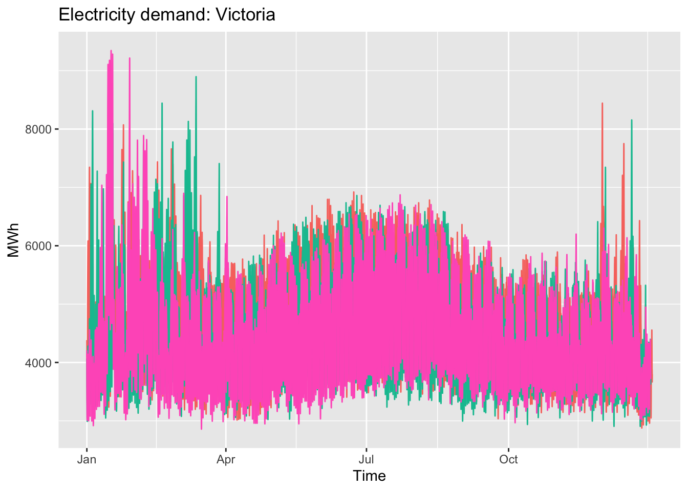
vic_elec |> gg_season(Demand, period = "year") +
  theme(legend.position = "none") +
  labs(y="MWh", title="Electricity demand: Victoria")

seasonal week plot:

Code

vic_elec |> gg_season(Demand, period = "month") +
  theme(legend.position = "none") +
  labs(y="MWh", title="Electricity demand: Victoria")

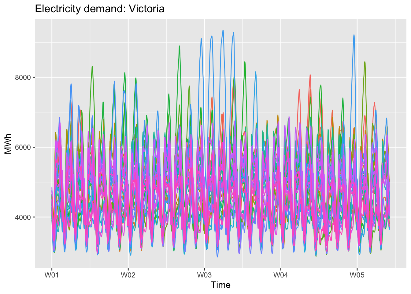
seasonal day plot:

Code

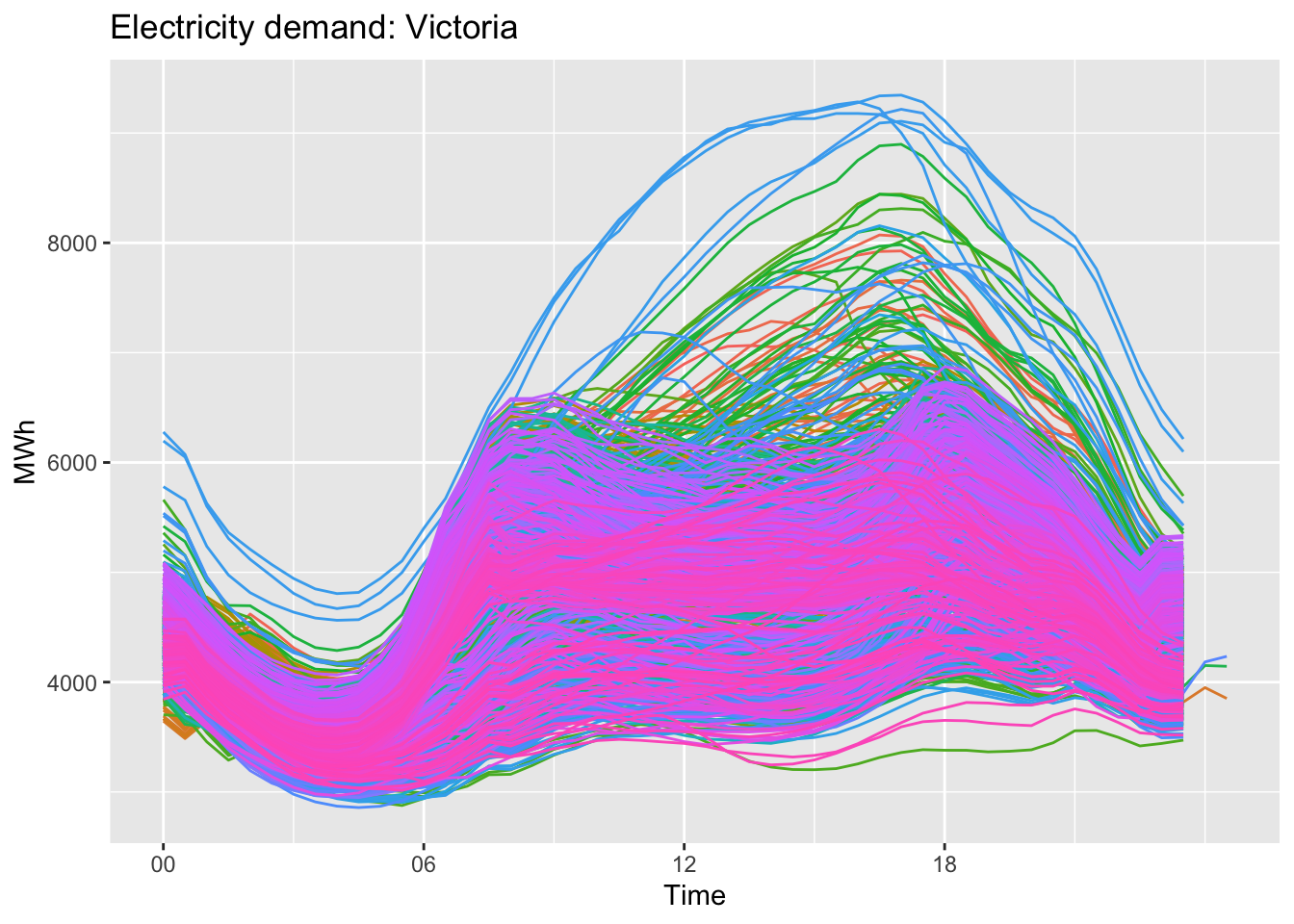
vic_elec |> gg_season(Demand, period = "week") +
  theme(legend.position = "none") +
  labs(y="MWh", title="Electricity demand: Victoria")

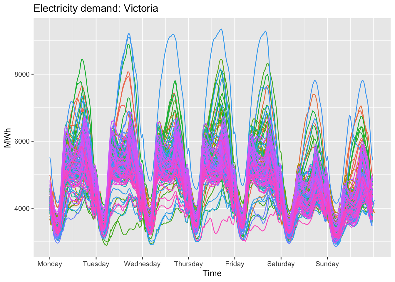
seasonal time plot:

Code

vic_elec |> gg_season(Demand, period = "day") +
  theme(legend.position = "none") +
  labs(y="MWh", title="Electricity demand: Victoria")

subseries plot:

Code

a10 %>% 
  gg_subseries(Cost) +
  labs(
    y = "$ (millions)",
    title = "Australian antidiabetic drug sales"
  )

3 Reference

https://fable.tidyverts.org/

https://otexts.com/fpp3/index.html

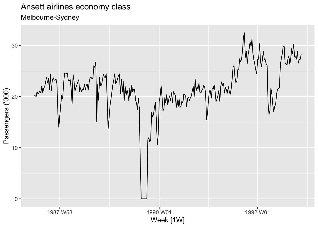
--- title: "time series analysis" author: "Tony Duan" date: "2023-08-30" categories: [packages] execute: warning: false error: false format: html: toc: true code-fold: show code-tools: true number-sections: true code-block-bg: true code-block-border-left: "#31BAE9" --- ![](images/Screenshot 2023-09-01 at 9.39.38 PM-01.png) The basic steps in a forecasting task: Step 1: Problem definition Step 2: Gathering information Step 3: Preliminary (exploratory) analysis Step 4: Choosing and fitting models Step 5: Using and evaluating a forecasting model ```{r} library(tidyverse) library(tidymodels) library(tsibble) library(tsibbledata) library(lubridate) library(dplyr) library(fpp3) ``` # data as tsibble convert data into tsibble ```{r} weather <- nycflights13::weather %>% select(origin, time_hour, temp, humid, precip) weather_tsbl <- as_tsibble(weather, key = origin, index = time_hour) ``` ```{r} head(weather_tsbl) ``` find index from tsibble ```{r} index(weather_tsbl) ``` find key from tsibble ```{r} key(weather_tsbl) ``` # plot time series data ```{r} melsyd_economy <- ansett %>% filter(Airports == "MEL-SYD", Class == "Economy") %>% mutate(Passengers = Passengers/1000) ``` ```{r} glimpse(melsyd_economy) ``` ```{r} autoplot(melsyd_economy, Passengers) + labs(title = "Ansett airlines economy class", subtitle = "Melbourne-Sydney", y = "Passengers ('000)") ``` ```{r} PBS |> filter(ATC2 == "A10") |> select(Month, Concession, Type, Cost) |> summarise(TotalC = sum(Cost)) |> mutate(Cost = TotalC / 1e6) -> a10 ``` ```{r} autoplot(a10, Cost) + labs(y = "$ (millions)", title = "Australian antidiabetic drug sales") ``` ```{r} glimpse(vic_elec) ``` seasonal month plot: ```{r} vic_elec |> gg_season(Demand, period = "year") + theme(legend.position = "none") + labs(y="MWh", title="Electricity demand: Victoria") ``` seasonal week plot: ```{r} vic_elec |> gg_season(Demand, period = "month") + theme(legend.position = "none") + labs(y="MWh", title="Electricity demand: Victoria") ``` seasonal day plot: ```{r} vic_elec |> gg_season(Demand, period = "week") + theme(legend.position = "none") + labs(y="MWh", title="Electricity demand: Victoria") ``` seasonal time plot: ```{r} vic_elec |> gg_season(Demand, period = "day") + theme(legend.position = "none") + labs(y="MWh", title="Electricity demand: Victoria") ``` subseries plot: ```{r} a10 %>% gg_subseries(Cost) + labs( y = "$ (millions)", title = "Australian antidiabetic drug sales" ) ``` # Time series components ```{r} us_retail_employment <- us_employment |> filter(year(Month) >= 1990, Title == "Retail Trade") |> select(-Series_ID) ``` ```{r} components(dcmp) |> as_tsibble() |> autoplot(Employed, colour = "gray") + labs(y = "Persons (thousands)", title = "Total employment in US retail") ``` ```{r} dcmp <- us_retail_employment |> model(stl = STL(Employed)) ``` ```{r} components(dcmp) ``` ```{r} components(dcmp) %>% autoplot() ``` read data and trend data ```{r} components(dcmp) |> as_tsibble() |> autoplot(Employed, colour="gray") + geom_line(aes(y=trend), colour = "#D55E00") + labs( y = "Persons (thousands)", title = "Total employment in US retail" ) ``` read data and trend+remainder(removed seasonal effect) data ```{r} components(dcmp) |> as_tsibble() |> autoplot(Employed, colour = "gray") + geom_line(aes(y=season_adjust), colour = "#0072B2") + labs(y = "Persons (thousands)", title = "Total employment in US retail") ``` # moving average ```{r} global_economy |> filter(Country == "Australia") |> autoplot(Exports) + labs(y = "% of GDP", title = "Total Australian exports") ``` ## 5 year moving average ```{r} aus_exports <- global_economy |> filter(Country == "Australia") |> mutate( `5-MA` = slider::slide_dbl(Exports, mean, .before = 2, .after = 2, .complete = TRUE) ) ``` ```{r} aus_exports |> autoplot(Exports) + geom_line(aes(y = `5-MA`), colour = "#D55E00") + labs(y = "% of GDP", title = "Total Australian exports") + guides(colour = guide_legend(title = "series")) ``` # Classical decomposition method two forms of classical decomposition: an additive decomposition and a multiplicative decomposition (developed in 1920s) ```{r} us_retail_employment |> model( classical_decomposition(Employed, type = "additive") ) |> components() |> autoplot() + labs(title = "Classical additive decomposition of total US retail employment") ``` # X11 method Its a multiplicative decomposition, whereas the STL and classical decompositions shown earlier were additive (developed in 1950s).Its only developed for quarterly and monthly data ```{r} # install.packages("seasonal") x11_dcmp <- us_retail_employment |> model(x11 = X_13ARIMA_SEATS(Employed ~ x11())) |> components() autoplot(x11_dcmp) + labs(title = "Decomposition of total US retail employment using X-11.") ``` # TRAMO/SEATS (developed in 1990s) ```{r} seats_dcmp <- us_retail_employment |> model(seats = X_13ARIMA_SEATS(Employed ~ seats())) |> components() autoplot(seats_dcmp) + labs(title = "Decomposition of total US retail employment using SEATS") ``` # STL(Seaonal and trend decompositiion) method its additive model. (developed in 1950s) ```{r} # robust = TRUE mean down weight (remove) outlier # window = "periodic" use all data us_retail_employment |> model( STL(Employed ~ trend(window = 7) + season(window = "periodic"), robust = TRUE)) |> components() |> autoplot() ``` default usual have good fit ```{r} us_retail_employment |> model( STL(Employed)) |> components() |> autoplot() ``` # Some simple statistics ```{r} tourism |> features(Trips, list(mean = mean)) |> arrange(mean) ``` ```{r} tourism |> features(Trips, quantile) ``` Autocorrelations ```{r} tourism |> features(Trips, feat_acf) ``` # forcast ## data preparation ```{r} gdppc <- global_economy |> mutate(GDP_per_capita = GDP / Population) head(gdppc) ``` ## data ploting ```{r} gdppc |> filter(Country == "Sweden") |> autoplot(GDP_per_capita) + labs(y = "$US", title = "GDP per capita for Sweden") ``` ## Define a model ```{r} TSLM(GDP_per_capita ~ trend()) ``` ## fit the model mable is model table ```{r} fit <- gdppc |> model(trend_model = TSLM(GDP_per_capita ~ trend())) fit ``` # Check model performance # Produce forecasts fable is forcast table ```{r} #forcast futher 3 years fit |> forecast(h = "3 years") ``` plot the forcast ```{r} fit |> forecast(h = "3 years") |> filter(Country == "Sweden") |> autoplot(gdppc) + labs(y = "$US", title = "GDP per capita for Sweden") ``` # some model ```{r} bricks <- aus_production |> filter_index("1970 Q1" ~ "2004 Q4") |> select(Bricks) ``` ## average model as benchmark ```{r} bricks |> model(MEAN(Bricks)) ``` ## Naïve method ```{r} bricks |> model(NAIVE(Bricks)) ``` ## Example: Australian quarterly beer production ```{r} # Set training data from 1992 to 2006 train <- aus_production %>% filter_index("1992 Q1" ~ "2006 Q4") # Fit the models beer_fit <- train %>% model( Mean = MEAN(Beer), `Naïve` = NAIVE(Beer), `Seasonal naïve` = SNAIVE(Beer) ) # Generate forecasts for 14 quarters beer_fc <- beer_fit %>% forecast(h = 14) # Plot forecasts against actual values beer_fc %>% autoplot(train, level = NULL) + autolayer( filter_index(aus_production, "2007 Q1" ~ .), colour = "black" ) + labs( y = "Megalitres", title = "Forecasts for quarterly beer production" ) + guides(colour = guide_legend(title = "Forecast")) ``` ## Google’s daily closing stock price ```{r} # Re-index based on trading days google_stock <- gafa_stock |> filter(Symbol == "GOOG", year(Date) >= 2015) |> mutate(day = row_number()) |> update_tsibble(index = day, regular = TRUE) # Filter the year of interest google_2015 <- google_stock |> filter(year(Date) == 2015) # Fit the models google_fit <- google_2015 |> model( Mean = MEAN(Close), `Naïve` = NAIVE(Close), Drift = NAIVE(Close ~ drift()) ) # Produce forecasts for the trading days in January 2016 google_jan_2016 <- google_stock |> filter(yearmonth(Date) == yearmonth("2016 Jan")) google_fc <- google_fit |> forecast(new_data = google_jan_2016) # Plot the forecasts google_fc |> autoplot(google_2015, level = NULL) + autolayer(google_jan_2016, Close, colour = "black") + labs(y = "$US", title = "Google daily closing stock prices", subtitle = "(Jan 2015 - Jan 2016)") + guides(colour = guide_legend(title = "Forecast")) ``` # Reference https://fable.tidyverts.org/ https://otexts.com/fpp3/index.html